Reduced AVL Tree
Distinguished professor Fabinaris Suchbaum and his team in Max Planck Institute for Software Systems in Saarbrücken are continuing their insightful investigations of binary search trees. This time they concentrate themselves on various variants of AVL trees. In the first phase, they want to study in detail the behaviour of the insert operation. To this aim they created a simplified version of AVL tree which they named Reduced AVL tree. It lacks the delete operation and it is equipped with so called reduce operation instead. The role of the reduce operation is to help keep the tree balanced and to partially simulate the missing delete operation. Another distinction of Reduced AVL tree is that any of its nodes can contain either one key or two keys.
Before we describe Reduced AVL tree, let us introduce some notation first.
Denote by Keys(X) the set of all keys in node X.
Denote by LCh(X), LSt(X), RCh(X), RSt(X),
the left child, the left subtree, the right child, the right subtree of node X, respectively.
Reduced AVL tree
Reduced AVL tree T is a binary rooted search tree. It is equipped with operations insert and reduce specified below
and it also satisfies the following five conditions.
- T1. Each node in T contains either one or two keys.
- T2. All keys in T are pairwise different.
- T3. Each node in T has either 2 or 0 children.
- T4. For each node X in T, the depths of LSt(X) and RSt(X) differ by at most 1.
- T5. For each internal node X in T, all keys in LSt(X) are smaller than min(Keys(X)) and all keys in RSt(X) are bigger than max(Keys(X)).
Denote by IK the key which is to be inserted. Insertion is performed by applying operation insert(IK, TR), where TR is the root of the tree. The operation insert(IK, X), where X is a node, is defined recursively by the following rules.
- I1. X is not defined (tree is empty). Create the root node of the tree and store IK in it. Stop.
- I2. IK = min(Keys(X)) or IK = max(Keys(X)). Stop.
- I3. X is an internal node, that is, both LCh(X) and RCh(X) exist.
- I3a. IK < min(Keys(X)). Apply insert(IK, LCh(X)).
- I3b. max(Keys(X)) < IK. Apply insert(IK, RCh(X)).
- I3c. min(Keys(X)) < IK < max(Keys(X)). Set K = min(Keys(X)), replace K by IK in X and apply insert(K, LCh(X)).
- I4. X is a leaf.
- I4a. |Keys(X)| = 1. Store IK in X. Stop.
- I4b. Keys(X) = {K1, K2}, K1 ≠ K2. Create two new nodes X1 and X2, set LCh(X) = X1, RCh(X) = X2. Distribute the keys IK, K1, K2 among the nodes X, X1, X2 in such way that each of these nodes contains exactly one key. Check if the tree is balanced and rebalance it if necessary, following the rules of standard AVL tree insert operation. Stop.
The operation reduce(T) changes the contents and the shape of T. Denote by RT the result of reduce(T). The properties of RT are:
- R1. RT is a Reduced AVL tree.
- R2. RT contains a key k if and only if k is a key stored in some internal node (non-leaf) in T.
- R3. The depth of all leaves in RT is the same.
- R4. Let A and B be two nodes in RT. If Keys(A) = {K1, K2}(K1 ≠ K2) and Keys(B) = {K3}, then max(K1, K2) < K3.
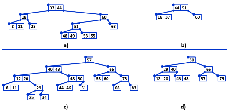 Image 1. Illustrations of the reduce operation. The Reduced AVL tree in Image 1b) is the result of applying reduce on the Reduced AVL tree in Image 1a). The Reduced AVL tree in Image 1d) is the result of applying reduce on the Reduced AVL tree in Image 1c). Note the positions of nodes with two keys
in 1b) and 1d). These are determined by the property R4 of the reduce operation.
Image 1. Illustrations of the reduce operation. The Reduced AVL tree in Image 1b) is the result of applying reduce on the Reduced AVL tree in Image 1a). The Reduced AVL tree in Image 1d) is the result of applying reduce on the Reduced AVL tree in Image 1c). Note the positions of nodes with two keys
in 1b) and 1d). These are determined by the property R4 of the reduce operation.
|
To test the behaviour of Reduced AVL trees the team formulated a simple additional rule which decides when the reduce operation has to be applied. Reduced AVL tree T is associated with two additional integer values RC and RCT. RC is a rotation counter and its value is initially 0. RC is increased by 1 each time a rotation occurs in the tree. Each double rotation (LR or RL) counts as one rotation in this case. RCT is a rotations counter threshold. It is a positive predefined constant. After each insert operation the equality RC = RCT is checked. If it holds then T := reduce(T) is performed and RC value is reset to 0.
The task
A value of RCT, an originally empty Reduced AVL tree T and a sequence of keys are given. Insert the keys into T. Determine the number of nodes in the resulting tree, the depth of the resulting tree and the number of reduce operations performed in the process.
Input
The first input line contains two integers N and RCT separated by space. N is the number of keys to be processed, RCT is a rotation counter threshold specified in the text. Each of the next N lines contains one integer key to be inserted into the Reduced AVL tree.
It holds 1 ≤ RCT ≤ N ≤ 2×10⁶.
Output
The output expects that all keys in the input were inserted into an initially empty Reduced AVL tree, in the same order in which they appear in the input. The output consists of one line containing integers NN, D, and R separated by spaces. NN is the number of nodes in the resulting tree, D is the depth of the resulting tree, R is the number of reduce operations performed in the process of inserting all given keys into the tree.
Example 1
Input9 1 22 11 12 77 55 88 33 44 66Output 3 1 1 |
Insert 33
   [12]_____
[11]        [55]
      [22,33]  [77,88]
......................
Insert 44
   [12]________
[11]         __[55]
         [33]     [77,88]
      [22]  [44]
.........................
Rotation R in node [55]
Rotation L in node [12]
       __[33]__
   [12]        [55]
[11]  [22]  [44]  [77,88]
.........................
-- Reduction --
   [33]
[12]  [55]
..........
Insert 66
   [33]
[12]  [55,66]
.............
Scheme 1. The tree in Example 1 in its final stages of developement. Link to a complete illustration of the tree developement. The illustrations are also included in the public data set below.
|
Example 2
Input21 2 30 27 29 21 23 20 24 16 14 25 12 15 19 51 52 53 54 55 56 57 12Output 5 2 2 |
Insert 56
             __[29]__
      [20,23]        [52]__
[14,16]     [25]  [51]     [54]
                        [53]  [55,56]
.....................................
Insert 57
             __[29]__
      [20,23]        [52]__
[14,16]     [25]  [51]     [54]__
                        [53]     [56]
                              [55]  [57]
........................................
Rotation L in node [52]
             __[29]________
      [20,23]            __[54]__
[14,16]     [25]     [52]        [56]
                  [51]  [53]  [55]  [57]
........................................
-- Reduction --
      [29,52]
[20,23]     [54,56]
...................
Insert 12
       __[29,52]
   [20]        [54,56]
[12]  [23]
......................
Scheme 2. The tree in Example 2 in its final stages of developement. Link to a complete illustration of the tree developement. The illustrations are also included in the public data set below.
|
Example 3
Input25 2 23 64 72 92 62 45 40 51 24 96 25 64 69 44 17 38 56 17 99 71 53 27 58 54 12Output 9 3 1 |
Insert 53
          ___________[45]___________
      [24]_____                   __[64]________
[17,23]        [40]           [56]            __[92]
         [25,38]  [44]  [51,53]  [62]     [71]     [96,99]
                                       [69]  [72]
..........................................................
Insert 27
          ______________[45]___________
      [24]________                   __[64]________
[17,23]         __[40]           [56]            __[92]
            [27]     [44]  [51,53]  [62]     [71]     [96,99]
         [25]  [38]                       [69]  [72]
.............................................................
Rotation R in node [40]
Rotation L in node [24]
                ________[45]___________
          __[27]__                   __[64]________
      [24]        [40]           [56]            __[92]
[17,23]  [25]  [38]  [44]  [51,53]  [62]     [71]     [96,99]
                                          [69]  [72]
.............................................................
-- Reduction --
          __[56]__
      [40]        [71]
[24,27]  [45]  [64]  [92]
.........................
Insert 58
          __[56]_____
      [40]           [71]
[24,27]  [45]  [58,64]  [92]
............................
Insert 54
          _____[56]_____
      [40]              [71]
[24,27]  [45,54]  [58,64]  [92]
...............................
Insert 12
             _____[56]_____
       __[40]              [71]
   [24]     [45,54]  [58,64]  [92]
[12]  [27]
..................................
Scheme 3. The tree in Example 3 in its final stages of developement. Link to a complete illustration of the tree developement. The illustrations are also included in the public data set below.
|
Public data
The public data set is intended for easier debugging and approximate program correctness checking. The public data set is stored also in the upload system and each time a student submits a solution it is run on the public dataset and the program output to stdout and stderr is available to him/her.
Link to public data set