Streak Binary Search Trees
The team of professor Fabinaris Suchbaum, located in Max Planck Institute for Software Systems in Saarbrücken, Germany, is studying various kinds of binary tree structures. In a typical search tree the number of keys in a node is either fixed or bounded by a fixed parameter. Trying to think out of the box, the team decided to perform some experiments on search trees in which the number of keys in a node is not limited.
Their idea of the so called streak BST is based on an obvious observation. When the keys are integers and the domain from which the keys are drawn is relatively small then it happens quite often that the search tree contains many pairs of keys which differ from each other by exactly one. It seems that it might be convenient to store both such keys in a single node. Of course, there may be much more than just two keys with the same property in the tree. This led the team to the definition of a streak.
Formally, a streak is a sequence of m (0 ≤ m) integer keys k1, k2, ..., km such that kj+1 = kj+1, (1 ≤ j < m).
Denote the streak by the symbol [k1...km].
A streak can also be empty (when 0 = m) or it may consist of a single value.
Storing a streak in a single node has an obvious advantage: No matter how long the streak is, any particular key in the node can be accessed in constant time.
The team has defined a streak BST and specified Insert and Delete operations in it.
A streak BST is a rooted binary tree T. For each node n in T it holds:
1. n contains an unempty streak [k1...km].
2. n.L.tree is either empty or it contains only values smaller than k1.
3. n.R.tree is either empty or it contains only values bigger than km.
4. T does not contain a key with value k1−1 or km+1.
Conditions 1. − 4. guarantee that each streak stored in the tree occupies a single node.
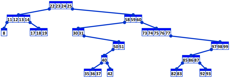 Image 1. An example of a streak BST with 15 nodes and 39 keys. The image illustrates Example 3 below before the last Delete operation is applied. |
Let us introduce some additional notation. Let n be a node in a streak BST.
Denote by n.tree the subtree which root is n.
Denote by n.L and by n.R the left child and the right child of n, respectively.
Denote by n.min and by n.max the respective values of k1 and of km in the streak [k1...km] stored in n.
If t is a subtree of a streak BST, denote by t.min and by t.max the value of the smallest key and the value of the biggest key in t, respectively.
Auxilliary operations used in the definition of Insert operation in a streak BST are LeftMerge and RightMerge.
LeftMerge. For each node n operation LeftMerge(n) is defined as follows.
If n.L.tree is empty the operation has no effect. Otherwise, let p be the node which contains the maximum key in n.L.tree. If p.max+1 = n.min move all keys from p to n and perform delete(p).
RightMerge. For each node n operation RightMerge(n) is defined as follows.
If n.R.tree is empty the operation has no effect. Otherwise, let p be the node which contains the minimum key in n.R.tree. If n.max+1 = p.min move all keys from p to n and perform delete(p).
Operation Insert
Insert operation is defined recursively for a streak K = [k1...km] and a node n. It is denoted by Insert([k1...km], n).
0. If the streak BST is empty, create a root node and store K in it.
1. If n.min ≤ k1 and km ≤ n.max stop, the operation has no effect.
Insert in L or R subtree:
2L. If km < n.min−1
If n.L.tree is empty create left child c of n and store K in c. Otherwise Insert(K, n.L).
2R. If n.max+1 < k1
If n.R.tree is empty create right child c of n and store K in c. Otherwise Insert(K, n.R).
Expand the streak in the node:
3. If k1 < n.min or n.max < km apply 3L or 3R or both, accordingly:
3L. If k1 < n.min delete([k1...n.min−1], n.L), store streak [k1...n.min−1] in n, LeftMerge(n).
3R. If n.max < km delete([n.max+1...km,] n.R), store streak [n.max+1...km] in n, RightMerge(n).
Operation Delete
Delete node. The operation delete node n works analogously to delete operation in ususal BST. It is denoted by Delete(n).
1. If n is a leaf remove n from the tree.
2. if n has just one child c remove n from the tree and make c a child of the parent of n. If n had no parent then make c the root of the tree.
3. The case when n has both children is handled separately in streak BST, see below.
Delete subtree. The operation delete subtree t removes all nodes in t from the streak BST. The operation is denoted by Delete(t).
Auxilliary operations used in the definition of Delete operation are LeftTrim and RightTrim specified below the description of Delete operation.
Delete operation is defined recursively for a streak K = [k1...km] and a node n. It is denoted by Delete([k1...km], n).
0. If node n is empty (or null) take no action.
Continue left or right:
1L. If km < n.min Delete(K, n.L).
1R. If n.max < k1 Delete(K, n.R).
Delete inside node:
2L. If km < n.max and k1 is equal to either n.min or n.min−1 delete streak [n.min...km] in n.
2R. If n.min < k1 and km is equal to either n.max or n.max+1 delete streak [k1...n.max] in n.
Delete inside node and continue deleting L/R:
3L. If k1 < n.min−1 and km < n.max delete streak [n.min...km] in n, Delete([k1...n.min−2], n.L).
3R. If n.min < k1 and n.max + 1 < km delete streak [k1...n.max] in n, Delete([n.max+2...km], n.R).
Delete inside node and move part of node keys to L/R subtree:
4. If n.min < k1 and km < n.max perform 4L or 4R accordingly.
4L. If k1 − n.min ≤ n.max − km delete streak [n.min...km] in n, Insert([n.min...k1−1], n.L).
4R. If k1 − n.min > n.max − km delete streak [k1...n.max] in n, Insert([km+1...n.max], n.R).
( Following cases 5. − 7. apply only when none of cases 1. − 4. applies.
In cases 5. − 7. the streak in the current node is a subset of the streak to be deleted. Parts of n.tree are deleted.)
Delete the whole subtree rooted in the node:
5. If k1 ≤ n.tree.min and n.tree.max ≤ km delete(n.tree).
Delete the node and optionally parts of its L/R subtrees:
6L. If k1 ≤ n.tree.min and km < n.tree.max delete(n.L.tree) delete([n.max+2...km], n.R), delete(n).
6R. If n.tree.min < k1 and n.tree.max ≤ km delete(n.R.tree) delete([k1...n.min−2], n.L), delete(n).
Delete node keys and relevant parts of both L and R subtrees:
7. If n.tree.min < k1 and km < n.tree.max
Do LeftTrim(n, k1).
Locate node y in n.L.tree containing n.L.tree.max. Delete all keys in n, copy all keys from y to n and Delete(y).
Do RightTrim(n, km).
LeftTrim(n, Val):
Delete in n.L.tree all nodes x such that Val ≤ x.min.
By deleting these nodes, the subtree n.L.tree is reduced to m (m ≥ 1) separate disconnected subtrees T1, T2, ..., Tm. Denote the roots of these trees by L1, L2, ..., Lm in ascending order of the root depths in original n.L.tree. For each j = 1, 2, ..., m−1 make Lj+1 the right child of the rightmost node in Lj.tree.
In Lm delete all keys bigger or equal to Val if such keys exist.
Set n.L = L1.
RightTrim(n, Val):
Delete in n.R.tree all nodes x such that x.max ≤ Val.
By deleting these nodes, the subtree n.R.tree is reduced to m (m ≥ 1) separate disconnected subtrees T1, T2, ..., Tm. Denote the roots of these trees by R1, R2, ..., Rm in ascending order of the root depths in original n.R.tree. For each j = 1, 2, ..., m−1 make Rj+1 the left child of the leftmost node in Rj.tree.
In Rm delete all keys smaller or equal to Val if such keys exist.
Set n.R = R1.
The task
You are given a sequence of Insert and Delete operations on an originally empty streak BST. Calculate the number of keys in each depth of the resulting tree.
Input
The first input line contains one integer N representing the number of sucessive operations performed on initially empty streak tree.
Next, there are N lines each of which describes one operation.
Each operation Inserts or deletes a streak of keys. The description starts with a single character "I" or "D" representing Insert or delete operation. Two integers kmin and kmax follow, representing the minimum and the maximum key in the streak, kmin ≤ kmax. All values on a line are separated by spaces.
It holds, 2 ≤ N ≤ 106. All keys are non-negative integers less than 105.
Output
The output contains two text lines. The first line contains the number of keys in the tree and the depth of the tree. The second line contains the numbers keys in consecutive depths in the tree, starting with the number of keys in depth 0. All values on both lines are separated by spaces. If the tree is empty the second line is empty. The depth of an empty tree is −1.
Example 1
Input6 I 50 60 I 70 75 I 74 80 I 10 20 I 30 40 D 15 55Output
21 1
5 16
*****  Insert 10...20
         [50...60]
[10...20]         [70...80]

*****  Insert 30...40
         _________[50...60]
[10...20]                  [70...80]
         [30...40]

*****  Delete 15...55
         [56...60]
[10...14]         [70...80]
Scheme 1. The tree in Example 1 in its final stages of developement. Link to a complete illustration of the tree developement. The illustrations are also included in the public data set below.
Example 2
Input9 I 0 99 D 49 50 D 24 25 D 37 37 D 31 32 D 34 34 D 10 12 D 6 7 D 13 23Output
76 5
49 2 17 5 2 1
*****  Delete 34...34
         ____________________________________[51...99]
[ 0...23]___________________________
                  __________________[38...48]
         [26...30]_________
                           [35...36]
                  [33...33]

*****  Delete 10...12
                  ____________________________________[51...99]
         [13...23]___________________________
[ 0... 9]                  __________________[38...48]
                  [26...30]_________
                                    [35...36]
                           [33...33]

*****  Delete 6...7
                           ____________________________________[51...99]
         _________[13...23]___________________________
[ 0... 5]                           __________________[38...48]
         [ 8... 9]         [26...30]_________
                                             [35...36]
                                    [33...33]

*****  Delete 13...23
                  ____________________________________[51...99]
         [ 8... 9]___________________________
[ 0... 5]                  __________________[38...48]
                  [26...30]_________
                                    [35...36]
                           [33...33]
Scheme 2. The tree in Example 2 in its final stages of developement. Link to a complete illustration of the tree developement. The illustrations are also included in the public data set below.
Example 3
Input16 I 22 25 I 11 14 I 58 60 I 8 8 I 17 19 I 30 31 I 73 77 I 50 51 I 97 99 I 40 40 I 82 93 I 35 37 I 42 42 D 84 84 D 88 91 D 23 41Output
30 5
1 7 11 4 3 4
*****  Delete 84...84
                  _________[22...25]_____________________________________________
         [11...14]                           ____________________________________[58...60]
[ 8... 8]         [17...19]         [30...31]___________________________                  [73...77]__________________
                                                               _________[50...51]                                    [97...99]
                                                      [40...40]                                             [85...93]
                                             [35...37]         [42...42]                           [82...83]

*****  Delete 88...91
                  _________[22...25]_____________________________________________
         [11...14]                           ____________________________________[58...60]
[ 8... 8]         [17...19]         [30...31]___________________________                  [73...77]___________________________
                                                               _________[50...51]                                    _________[97...99]
                                                      [40...40]                                             [85...87]
                                             [35...37]         [42...42]                           [82...83]         [92...93]

*****  Delete 23...41
                  _________[22...22]__________________
         [11...14]                                    [58...60]
[ 8... 8]         [17...19]                  [50...51]         [73...77]___________________________
                                    [42...42]                                             _________[97...99]
                                                                                 [85...87]
                                                                        [82...83]         [92...93]
Scheme 3. The tree in Example 3 in its final stages of developement. Link to a complete illustration of the tree developement. The illustrations are also included in the public data set below.
Public data
The public data set is intended for easier debugging and approximate program correctness checking. The public data set is stored also in the upload system and each time a student submits a solution it is run on the public dataset and the program output to stdout and stderr is available to him/her.
Link to public data set